Lyapunov Stability

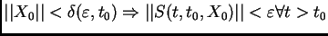
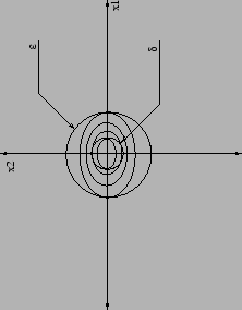
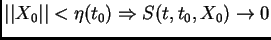
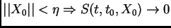
Definition 5.1.1   Stability The equilibrium is stable if for each $\varepsilon >0$ and each $t_{0} \epsilon \mathbb{R}_{+}$ there exists a

$$\delta = \delta (\varepsilon ,t_{0})$$ (5.1)

such that

$$\vert\vert X_{0}\vert\vert < \delta (\varepsilon ,t_{0}) \Rightarrow \vert\vert S(t,t_{0},X_{0})\vert\vert<\varepsilon \forall t>t_{0}$$ (5.2)

where
$X_{0}$ is the initial Condition. $S(t,t_{0},X_{0})$ is the solution trajectory (Starting from initial condition and initial time $t_{0}$)

It is uniformly stable if for each $\varepsilon >0$ there exists $\delta =\delta (\varepsilon )$ such that $\vert\vert X_{0}\vert\vert<\delta (\varepsilon )\Rightarrow \vert\vert S(t,t_{0},X_{0})\vert\vert\leq \varepsilon \forall t\geq t_{0}$.

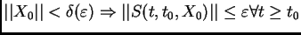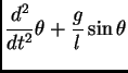
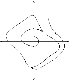
Example 5.1.1  

$$\frac{d^{2}}{dt^{2}}\theta + \frac{g}{l}\sin \theta =0 ; \theta =0,\pi ,2\pi \ldots$$ (5.3)

$$x_{1} = \theta$$ (5.4)

$$\frac{dx_{1}}{dt} = x_{2}$$ (5.5)

$$\frac{dx_{2}}{dt} = -\frac{g}{l}\sin \theta$$ (5.6)

Figure 5.1: Stable Equilibrium

Example 5.1.2  

$$\frac{dx_{1}}{dt} = x_{2}$$ (5.7)

$$\frac{dx_{2}}{dt} =x_{1}+(1-x_{1}^{2})x_{2}$$ (5.8)

Figure 5.2: Unstable Equilibrium

no $\delta$ can be found for this $\varepsilon$. If we take $\varepsilon$ sufficiently large to contain the limit cycle then we can find a $\delta$ which satisfies the stablity criterion but is should be true for each and every $\delta$.

Definition 5.1.2   The equilbrium $\overline{0}$ is attractive if for each $t_{0} \in \mathbb{R}_{+}$ there is $\eta (t_{0})>0$ such that

$$\vert\vert X_{0}\vert\vert<\eta (t_{0})\Rightarrow S(t,t_{0},X_{0})\rightarrow 0 t \rightarrow \infty$$ (5.9)

Definition 5.1.3   It is uniformly attractive if there is $\eta >0$ such that

$$\vert\vert X_{0}\vert\vert<\eta \Rightarrow S(t,t_{0},X_{0})\rightarrow 0$$ (5.10)

as $t\rightarrow \infty$ uniformly in $t_{0},X_{0}$

Attractivity doesn't imply stability and vice versa. Another Definiton of stability: Asymptotic Stability

Definition 5.1.4   Equilibrium $\overline{0}$ is uniformly asymptotically stable if it stable and attractive.

Definition 5.1.5   Equilibrium $\overline{0}$ is uniformly asymptotically stable if it is uniformly stable and uniformly attractive.

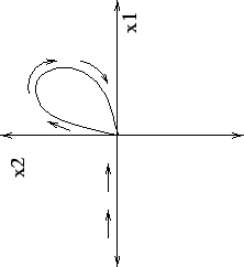
Example 5.1.3   Vinograd's Equation (1957)

$$\frac{dx_{1}}{dt} = \frac{x_{1}^{2}(x_{2}-x_{1})+x_{2}^{5}}{x_{1}^{2}+x_{2}^{2}[1+(x_{1}^{2}+x_{2}^{2})^{2}]}$$ (5.11)

$$\frac{dx_{2}}{dt} =\frac{x_{2}^{2}(x_{2}-2x_{1})}{(x_{1}^{2}+x_{2}^{2})[1+(x_{1}^{2}+x_{2}^{2})^{2}]}$$ (5.12)

equilibrium $\equiv (0,0)$

Figure 5.3: Not Stable but attractive

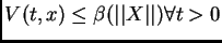
Definition 5.1.6   Exponentional Stability
Equilibrium $\overline{0}$ is exponentionally stable if there exists constants $r,a,b>0$ such that

$$\vert\vert S(t,t_{0,}X_{0})\vert\vert\leq a\vert\vert X_{0}\vert\vert e^{[-b(t-t_{0})]}$$ (5.13)

for all $t>t_{0}$ and $x_{0}\epsilon B$

All the linear systems if they are stable, they an exponentially stable.

Definition 5.1.7   Global Uniform Asymptotic Stability
Equilibrium $\overline{0}$ is globally uniformly asymptotially stable if

• It is uniformly stable
• For each pair of positive numbers $M,\varepsilon$ with $M$ arbitrarily large and $\varepsilon$ arbitrarily small there exists a finite number $T=T(M,\varepsilon )$ such that $\vert\vert X_{0}\vert\vert<M$, $t_{0}\geq 0 \Rightarrow \vert\vert S(t,t_{0},X_{0})\vert\vert<\varepsilon$ for all $t>T(\varepsilon ,M)$

Definition 5.1.8   it Function of Class K and Class L
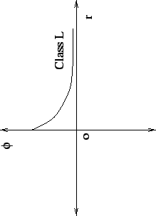
Function $\phi : \mathbb{R}_{+}\rightarrow \mathbb{R}_{+}$ is of class K if it is continuous, strictly increasing, and $\phi(0) = 0$. It is class L if it is continuous on $[0,\infty)$ strictly decreasing, $\phi (0)<\infty$, $\phi(r) \rightarrow 0$ as $r\rightarrow \infty \protect$

Figure 5.4: Class K

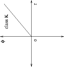Figure 5.5: Class L

Definition 5.1.9   Definition:Locally Positive Definite Function and Positive Definite Function
A function $V : \mathbb{R}_{+} \times \mathbb{R}^{n}\rightarrow \mathbb{R}$ is said to be locally positive definite function/positive definite function:(lpdf)/(pdf)

• It is continuous.
• $V(t,0)=0 \forall t\geq 0$
• then exists a constant $r>0$ and function $\alpha$ of class K such that $\alpha \vert\vert X\vert\vert\leq V(k,x) \forall t\geq 0$ and $X\epsilon B_{r}^{*}(\mathbb{R}^{n})$ for lpdf(pdf)

V is decrescent if there exists a constant $r>0$ and a function $\beta$ of class K such that $V(t,x)\leq \beta (\vert\vert X\vert\vert) \forall t>0$ and $X\epsilon B_{r}$ V is radially unbounded if * is satisfied for some $\alpha _{1}$ (not necessarily class K) with additional property $\alpha _{1}(r)\rightarrow \infty$ as $r\rightarrow \infty \protect$

Figure 5.6: Radially Unbounded