


Next: Analyse the following system
Up: 14/01/2003 by Ajit Shegaonkar
Previous: 14/01/2003 by Ajit Shegaonkar
Consider the folowing block diagram :-
Figure 1.1:
Rocket Control
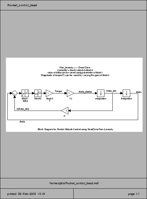 |
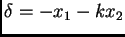
The state space variables are :-
For the Controller , the control action can be represented as :-
 |
(1.3) |
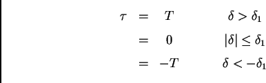 |
(1.4) |
where  is the torque applied.
From the above equations, the equations of the switching lines are :-
is the torque applied.
From the above equations, the equations of the switching lines are :-
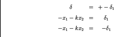 |
(1.5) |
The Trajectories are as shown in the figure below :-
Trajectory1
As compared to the system containing controller without the dead-zone, this system will have lesser fuel consumption but at the same time, it may not give the shortest time required to reach the equillibrium point.
Another way of controlling the rocket is by using a controller having
memory where the controller non-linearity is positive Hysteresis. (Assignment)


Next: Analyse the following system
Up: 14/01/2003 by Ajit Shegaonkar
Previous: 14/01/2003 by Ajit Shegaonkar
Vishal Mahulkar (98D10043)
2003-02-14